Demand Curves are Cumulative Distribution Functions (CDFs)

Aggregations as accumulations

(Epistemic Status: A simple point meant to help when thinking about demand curves. No serious new insight is claimed on my part, but I do not remember having seen a similar analysis. I think all of this makes sense, but I haven’t actually ‘done the math,’ so it could be broken in some way.)

I would consider myself a decent student of economics, but one area I have struggled with is the shape of the demand curve. In particular, I have found it difficult to get an intuitive grasp on how manipulations in the shape of the demand curve should change my expectations about the market (or vice versa) beyond generalized changes in elasticity/responsiveness to market shifts. Now, having spent some time thinking about the topic, I believe I have found a more intuitive way to understand/present some aspects (including the shape) of the demand curve.

Valuation Distributions

To understand how the method operates, I think it is probably easiest to begin at the end and work backward.

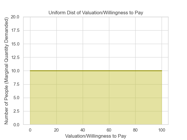
To start, we will construct a valuation or ‘willingness to pay’ distribution for the population. For the sake of simplicity, we will assume a thousand people with valuations uniformly distributed from one to one hundred. We will also assume that all prices and valuations are in whole dollars. And that each person only wants to buy one item. If we do this, then we get the distribution pictured below, where there are ten people with each dollar valuation from one to one hundred. Ten people with a valuation of one dollar, ten people with a valuation of two dollars, and so on.

Now that we have this distribution of valuation, we can add in a ‘current price’ (set to $80 in the graph below). People with valuations greater than a given ‘current price’ (i.e., those to the right of the price line in the graph below) are able to successfully buy the item at that price, while those below the price cannot.

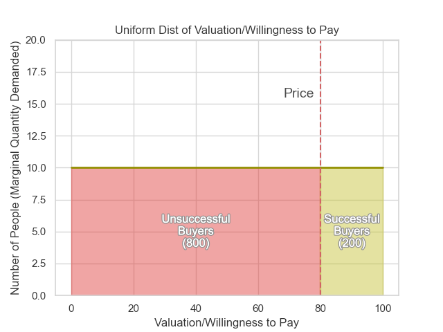
We can observe from the analysis above that the number of items sold at the ‘current price’ is equal to the greenish area under the curve. This is because for every valuation above the ‘current price, ’ all ten of the individuals with that valuation will buy an item.¹

Indeed, if we examine this more closely, it becomes clear that the number of items successfully sold will always be equal to the area under the right side of the curve, which is to say the integral between the price and the highest valuation (or positive infinity, if you want). This is true for any valuation distribution.

Constructing the Cumulative Distribution Function (CDF)

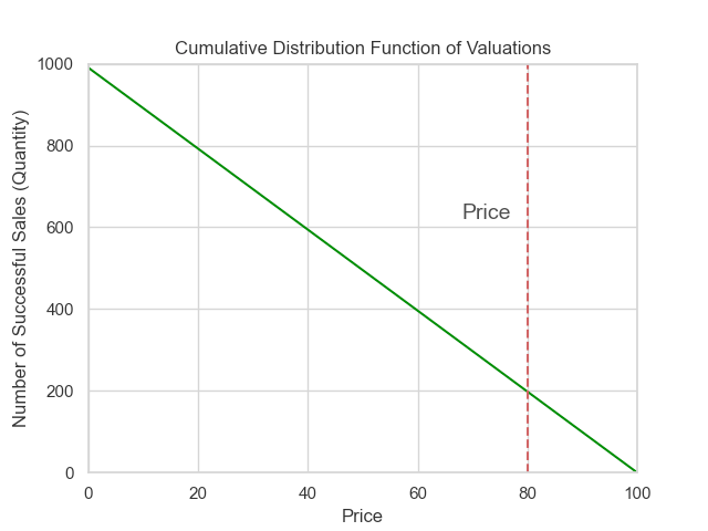
If you are familiar with probability theory, you might recognize that what we just described is actually a scaled Cumulative Distribution Function (CDF)² for the Uniform distribution (the population distribution we picked).

Given that correspondence, we can just read off the CDF of the uniform distribution.

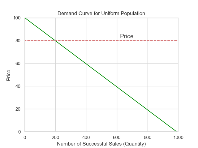
Now that we can see the CDF function, it is trivial to convert it into a classic demand curve. All we have to do is switch the axes.

From this process, a few things are hopefully clear:

1. A demand curve is approximately mathematically equivalent to a distribution of valuations.

2. It is relatively easy to convert from a distribution of valuations to a demand curve (integrate and swap axes) and from a demand curve to a distribution of valuations (the inverse: swap axes and differentiate).

3. Classic linear demand curves of the form P = a - bQ imply a uniform distribution of valuations.

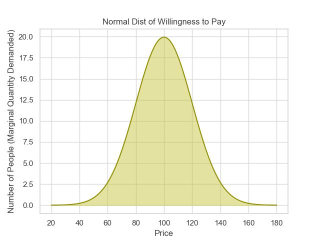
At this point, you might be wondering whether this is actually a useful method for understanding demand. Fortunately, I think I have an interesting question that only this kind of analysis can easily pose and answer, namely, “what is the demand curve of a normally distributed set of valuations?”

Normieconomics

To answer this question, we just need to use the same strategy as before. First, we get our valuation distribution:

Then, we construct the CDF for that distribution (which is the same as the area under the curve/the integral we need):

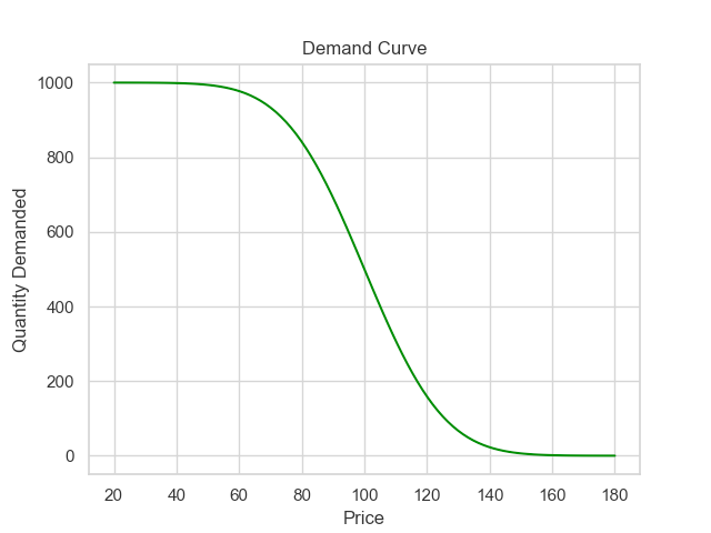
Next, we swap the axes for the CDF so that it becomes a demand curve. Here, I think it’s worthwhile to display the valuation distribution on a shared axis with the demand curve (as I’ve done below) so that the relationship between the two is clearer.

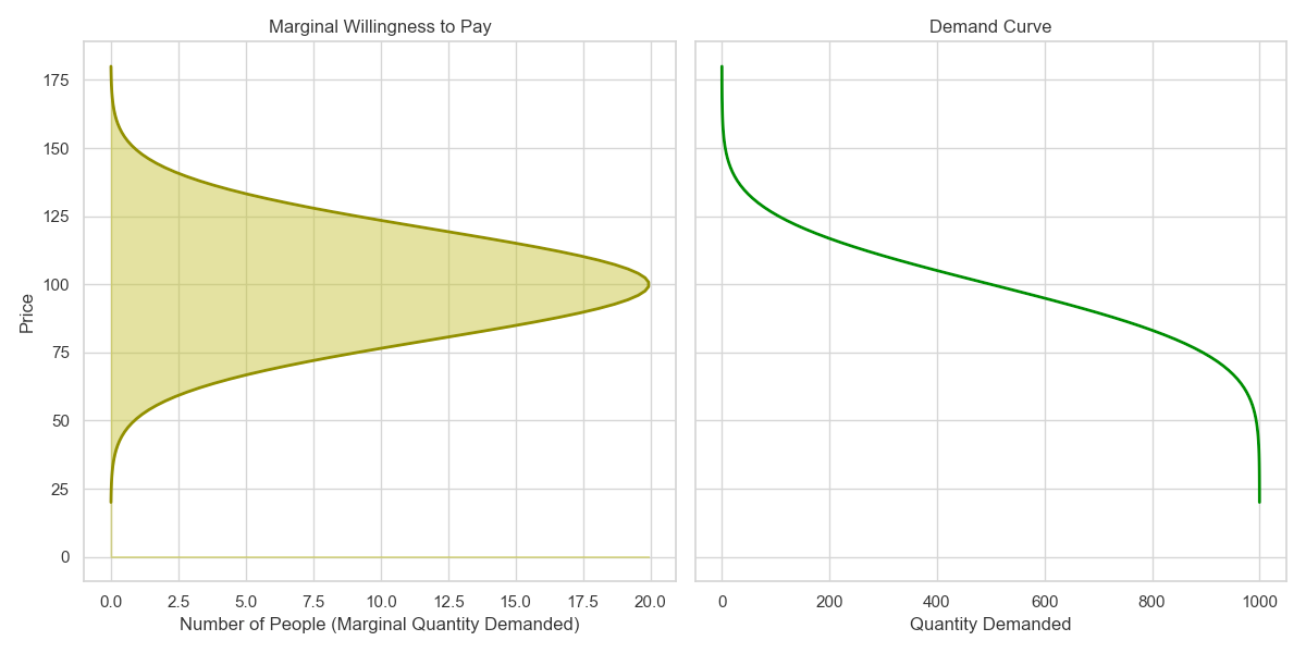
And there you go! The demand curve of a normal distribution is a weird sigmoid! This is not particularly surprising, but interestingly, it does seem like the middle ~80% of the demand curve actually resembles a simple linear demand curve.

Final Thoughts

• In both of my examples, I started with the population valuation distribution, but I expect that this is likely just as useful in the other direction.

• I think that placing the valuation distribution and the demand curve on a shared axis is probably the best thing to do since it lets you freely convert between the two kinds of graphs. It also lets you see how they relate to each other.

• The choice of the uniform and normal distributions as examples was not random. Regarding the uniform dist, I think it is important to highlight that the common linear demand curves seen in undergraduate coursework include an implicit (and obviously simplifying) assumption of a uniform distribution of valuations. Regarding the normal distribution, I think that the normal distribution seems quite plausible for some simple markets. Of course, I may be wrong, in which case I defer to whatever the empirical findings are.

• In my examples, I assumed that individuals only wanted one item so that the valuation distribution matches the human distribution more straightforwardly. If we let people buy more items, then the valuation distribution needs to include valuations for multiple items from the same person. This is fine and continues to match the demand curve, but it is a bit more complicated to reason about.

• The reason the demand curve is a CDF is that as you lower the price, all of the previous buyers stay accumulated. This is equivalent to the Law of Demand, but sometimes the law of demand is violated (such as for Giffen goods), in which case this analysis also breaks down to some extent.³

Anyway, that’s it! Let me know if you have any thoughts or comments.

Recommendations

This post’s (unrelated) recommendations are:

• ‘You can’t take it with you: straight talk about epigenetics and intergenerational trauma’ by Razib Khan

  • Razib explains both the incredible power and wonder of epigenetics and how popular science claims that trauma is inheritable are completely unfounded.

• “TrueSkill Part 1: The Algorithm” by DJ Rich

  • The post explains the TrueSkill algorithm developed by Microsoft for matchmaking, invented in response to limitations of the Elo scoring system from chess. The algorithm is pretty interesting and can robustly incorporate a lot of different features.

  • The second post in the series ‘TrueSkill Part 2: Who is the GOAT?’ uses the TrueSkill algorithm to find the GOAT player for Tennis, Boxing, and Warcraft 3.

  • If you have the time and interest, I highly recommend reading/watching everything on the True Theta blog and the associated YouTube channel (not that I’ve managed it yet myself). Lots of fascinating stuff I haven’t seen elsewhere.

1. This assumes that the Law of Demand holds. This is a load-bearing assumption for this analysis, but it is so rarely violated that I have left mention of it to this footnote and the final thoughts section.

2. Or rather one minus the CDF, since we are moving from right to left instead of the normal left to right).

3. You can still generate the same type of graph, but you will need to have ‘negative’ items for certain valuations, which is a bit weird to reason about.