
Optimal Deterrence
Matching the punishment to the criminal

(Epistemic status: Pure theory. Ideas are very worth considering, but they are likely trumped by other factors in practice.)
The law is full of nonsense. Indeed, it is so full of clear and obvious nonsense that simple questions can be made to seem unanswerable merely by association. One such question is ‘How much should a person be punished for breaking the law?’ Today I’ll try to partially answer that question, potentially with some unintuitive results.
Before beginning, I will note that punishment, especially incarceration, is typically characterized as having three ‘benefits,’ namely retribution, incapacitation, and deterrence. However, I will only be considering the implications of deterrence. In the case of retribution, I simply don’t consider it a benefit. In the case of incapacitation, I consider it to be separate from punishment itself. This is because the purpose of incapacitation is to physically prevent future crimes, not to punish past ones, and because such prevention can potentially occur without any notable harm to the future offender.
What costs/benefits?
In order to determine the optimal punishment for a crime, I will be weighing, on the one hand, the benefits of deterring crime, and, on the other hand, the costs of inflicting harm on offenders. If you are unwilling to consider the welfare of criminal offenders, then you can substitute in some other rule-breaking context, such as students breaking rules in a school or children breaking their parents’ rules, where the punished individuals are more sympathetic. The model should still apply regardless.
Building the Deterrence Model
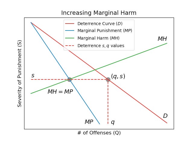
One basic feature we should expect from our model is that, as threats increase in severity, the number of offenses should decrease and vice versa. Graphing this results in something very similar to a demand curve for offenses, with severity of punishment as the price.
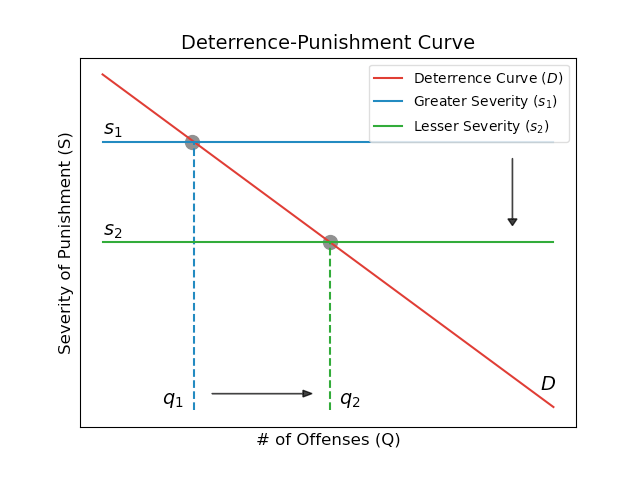
We can then observe that for a given level of punishment (S), the total harm inflicted is the severity of punishment (S) multiplied by the number of offenses punished (Q).
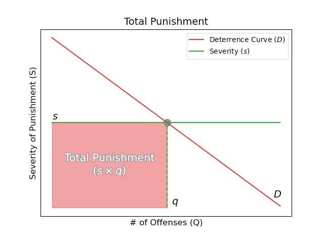
As a result, raising or lowering the severity of punishment (S) can have different effects on total punishment (s x q) depending on the current number of offenses (Q). To simplify this relationship, we can calculate a Marginal Punishment (MP) curve for the cost of raising/lowering the severity of punishment (S). This curve is the actual effect of a marginal change in the severity of punishment (S) on total punishment, including both the effect on the number of offenses and the effect on the degree of punishment for those offenses.
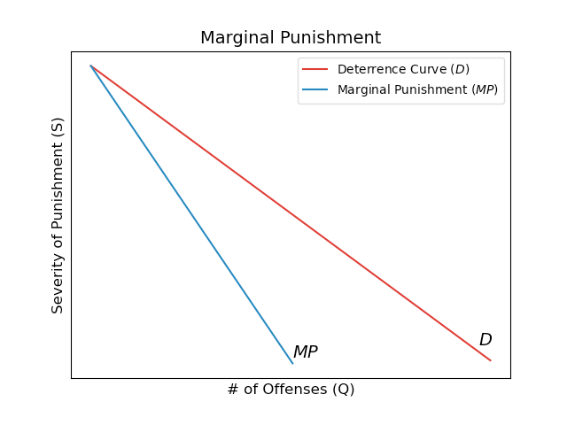
Now that we have a Marginal Punishment (MP) curve to serve as our marginal cost curve, all we need now is to include a marginal benefit curve from prevented crimes and then we can calculate the optimal deterrence severity (S).
Constant Harm Case
To start out, we can consider the relatively simple case where offenses have a constant degree of harm. Given the marginal harm, we can now find the optimal point where marginal cost is equal to marginal benefit, i.e. where marginal punishment (MP) is equal to the harm of a marginal offense (MH).
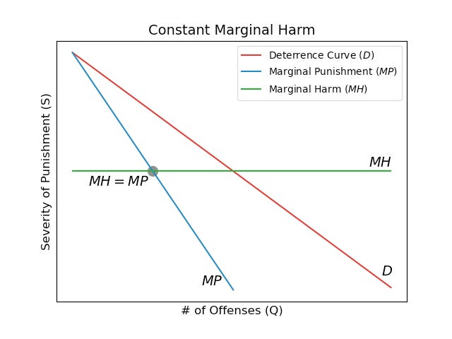
In this case, we get the fairly intuitive conclusion that the optimal severity of punishment (S) for each offender should be equal to the harm of their offense (MH).
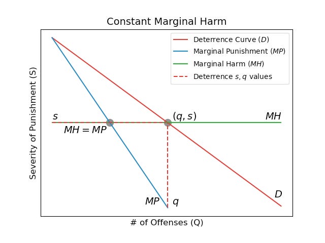
This kind of model seems likely to describe many real offenses, especially when the offenses are generally committed in isolation and when individuals are generally only victimized once. Pickpocketing, for example, if diffused across a city, likely has an approximately constant marginal harm.
Decreasing Harm Case
Next, we can consider a more interesting case, where marginal harm is decreasing.
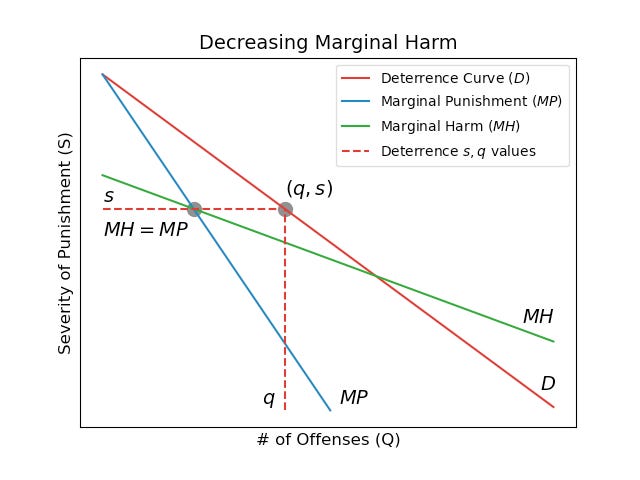
Looking at the graph for this scenario, the most notable feature is that the severity of punishment (S) is greater than the marginal harm (MH). This fact is not necessarily obvious if you haven’t spent time studying similar graphs in economics, so I’ll try a quick explanation.
Graphical Explanation
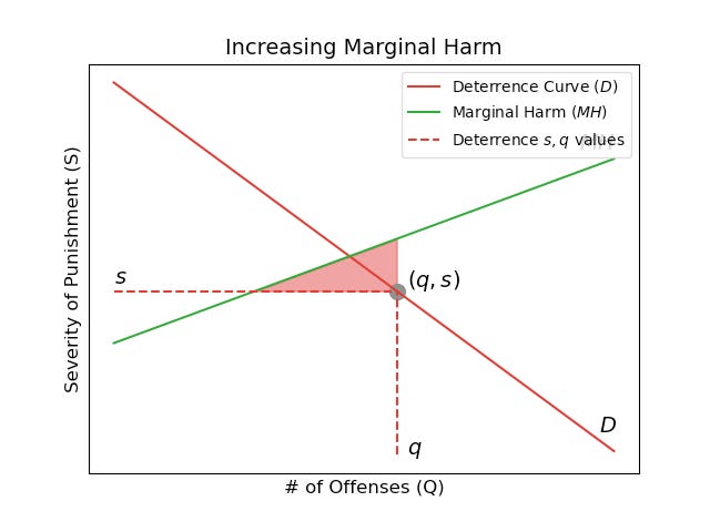
The first point to note is that once the optimal punishment (S) is determined (MH=MP), we can ignore the marginal punishment (MP) curve. Once we remove it, we get this graph:
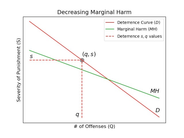
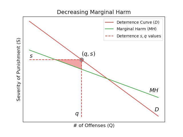
Looking at this graph we can see that the marginal offense occurs at the vertical dashed line ‘q’. In this case, the marginal harm of the offense is equal to the green line at ‘q’, while the punishment the offender receives is equal to the horizontal dashed line ‘s’. With this in mind, we can observe that the marginal harm (green line) is less than the severity of punishment (horizontal dotted line) at the current margin (vertical dotted line). This means that the marginal offender is punished more than the harm they actually caused. Indeed, the whole area between the marginal harm curve and the severity (‘s’) line represents cases where the offender’s punishment is more severe than the harm they caused.
Practical Meaning
So why does it make sense for offenders to be punished more than the harm they cause and when would a model like this apply? Some people may be able to just intuit answers from the graphs above, but for the rest of us, I will try to explain through an example.
One case where this kind of model plausibly applies is throwing soup on the Mona Lisa (unprotected this time), or, if you want a less controversial example, graffitiing on building walls. To begin with, we can imagine that there is no punishment for the offense (i.e. no deterrence) and that fifteen people are willing to throw soup on the Mona Lisa and/or graffiti the wall of a building. If we think clearly about this, it is obvious that the fifteenth person throwing soup on the Mona Lisa and/or graffitiing the wall is having much less effect than the first, second, or even third person. This results in a situation where the individuals who it is most difficult to deter (e.g. the first, second, and third) are the most valuable to deter and the individuals it is easiest to deter (e.g. the thirteenth, fourteenth, or fifteenth) are the least valuable to deter. Since the value of deterrence is increasing as deterrence increases, it becomes worthwhile to trade some extra increases in total punishment for increases in deterrence at the margin.
Increasing Harm Case
Since we’ve examined the decreasing harm case, it is natural to next consider the increasing harm case.
Working through this case, the conclusions are generally the reverse of what was found in the decreasing harm case. In particular, the marginal harm curve (MH) now exceeds the severity of punishment (‘s’) at the margin, so marginal offenders (at ‘q’) are punished less than they harm society, rather than more. Of course, as before, this is true for more than just the exact marginal offender.
Practical Meaning
As before, it's worth working through an example to show where this kind of model would apply and how it makes sense. For this, we can consider the case of fraud committed by members of asset rating agencies. To understand why the model applies, we can observe that if an individual asset analyst commits fraud, perhaps by marking a mortgage security as safer than it really is, then the asset’s buyer will potentially lose more on that asset than expected, but overall we should expect the harm to be somewhat limited. However, if a large number of analysts all start committing such fraud, the market can be severely destabilized by unexpected correlated failures, potentially even creating a financial crisis. In such a case, the one-hundredth person committing fraud can do substantially more harm than the first person committing fraud. This results in a situation where the individuals who it is easiest to deter (e.g. the ninety-eighth, ninety-ninth, and one-hundredth) are the most valuable to deter and the individuals it is most difficult to deter (e.g. the first, second, or third) are the least valuable to deter. Since most of the benefit comes from deterring offenders who are easier to deter, there is less reason to raise the severity of punishment to deter offenders who are more difficult to deter.1
Is This Really Optimal Deterrence?
There are a number of simplifying assumptions that went into the models above (no enforcement costs, perfect true-positive detection, etc.) that I expect can be updated/made more realistic without fundamentally altering the conclusions above. However, there is another implicit and perhaps non-obvious assumption that is fundamental to the analyses, namely the assumption that every offender must be punished with the same severity. In economics terminology, this means the state is not engaging in ‘price discrimination’ for offenders.
The fact that the severity of punishment must be consistent across offenders is what creates the divergence between marginal punishment (MP) and the deterrence curve (D) in the model. The reason the marginal punishment curve is steeper than the deterrence curve is that increasing the severity of punishment for one offender requires increasing the severity for all the other remaining offenders. As a result, the total increase in severity is multiplied by the number of remaining offenders and rises faster.
However, if we stop requiring that offenders be punished equally, then (in a perfect information world) marginal punishment (MP) can be made equal to the deterrence curve (D). Such an equivalence makes the ‘increasing harm’ and ‘decreasing harm’ cases above uninteresting, since there is no reason to punish any offender either more or less than is necessary to deter them. Indeed, each individual could be considered entirely in isolation and have a personally tailored punishment, set just high enough that they will never offend.
The Undeterred
I’m sure that by the end of my previous sentence, many readers were objecting to the hypothetical where everyone could be convinced not to offend. On this point, I entirely agree. Some offenses cannot be deterred due to irrationality, ignorance, or insufficient punishment capabilities. In such cases, a state engaging in ‘price discrimination’ should simply not punish those individuals. To do so would just harm people for no reason.
This may seem somewhat strange, but I consider it to be the underlying reason why insanity is an acceptable defense in court. Additionally, it is important to note here that I am not considering incapacitation as part of punishment. For example, even if an ‘insane’ individual should not be punished for their actions, it can still be reasonable to institutionalize them to avoid future offenses. Indeed, such incapacitation is so divorced from punishment that it can reasonably be used even when no crime has yet occurred, such as in the case of involuntary commitment.
Final Thoughts
To end this, I’ll just note some closing thoughts:
The kind of ‘price discrimination’ system described above might appear far-fetched. However, it is essentially the same logic underlying Finland and Switzerland’s speeding ticket systems, which take a person’s salary into account when calculating fines. Those systems do not necessarily vindicate the ideas presented, but they do show how such ideas are possible in the real world.
Even if the state is not able to perfectly ‘price discriminate’, efforts to improve ‘price discrimination’ are likely to improve outcomes. For example, the existence of juvenile courts can be seen as a form of ‘group pricing’ (third-degree price discrimination). Escalating punishments for repeat offenders is similarly a way to increase punishments for a group who are undeterred by the current level of punishment.
As long as ‘price discrimination’ by the state is imperfect, the imperfections described in the sections on increasing and decreasing harms will persist.
The model of deterrence described here is not limited to criminal contexts and could easily be applied to a number of different environments.
The point of this post is theoretical exploration, not real-world recommendations. I don’t know enough about the empirics of crime to have a strong opinion.
I believe there are some strong objections to this kind of ‘price discrimination’ in practice, particularly in the vein of principal-agent problems and tax collection incentives. However, I am skeptical that rich people should get to speed more because their time is more valuable, as Tyler Cowen has claimed. There is a distinction between economic welfare and utility and at some level, utility must dominate.
P.S. Following Dynomight’s blog, I’ve decided to start including a couple of links to writing I thought was particularly good at the end of my posts.
A computer science-y choice: ‘NP-Complete isn't (always) Hard’ by Hillel Wayne
Pointing out that big O is worst-case analysis, not average, plus some more interesting notes.
A general science choice: ‘Quick look: applications of chaos theory’ by Elizabeth Van Nostrand and Alex Altair
Investigating whether/where chaos theory is actually used. A good companion piece to the James Gleick ‘Chaos’ book.
Follow-up post.
Does this justify the notoriously light punishments faced by members of the financial industry after the financial crisis? I am very skeptical, but you could make the argument.