
What can you do with barely any data?
Simple median finding with few datapoints

(Epistemic Status: Exploring a cool technique I came across. Usefulness is debatable, but plausibly decent if you need something you can do in your head. Some of the math is intentionally handwavey, but I think the basic points are robust.)
A little while ago, I was reading How to Measure Anything by Douglas Hubbard. For the most part, I found that the book, though interesting, mainly covered ideas and concepts I already knew, such as ‘value of information’, A/B testing, linear regression, and Bayesian forecasting. However, there was one fascinating exception that, after learning, I felt I had to share and investigate, thanks to its remarkable combination of incredible simplicity and strong mathematical guarantees.
The Method
The method, as I said, is remarkably simple. To understand it, we can first ask the question: What is the probability that n random, independently chosen samples are all above the population median? The answer to this question is pretty straightforward. Since there is a one-half chance that a single sample is above the median (by the definition of the median1), the probability that all of the independent samples are above the median is ½ raised to the power of n: (½)n.
Taking this result, we can then say, by symmetry, that the probability that n random, independently chosen samples are all below the population median is also ½ raised to the power of n: (½)n.
Now, since both of these possibilities are mutually exclusive, we can say that the probability that either all the n samples are above the median or all the n samples are below the median is just the sum of the two individual probabilities, which is just ½ raised to the power of n minus one: (½)n-1.
This result might not seem particularly interesting, but if we switch to describing the complement (i.e., the event that neither of the conditions above is true), then this takes on a very different meaning. Specifically, it says that for n random, independently chosen samples, the probability that at least one sample is above the median and that at least one sample is below the median is one minus our combined probability from before.2 This means that, if you take the range between the sample maximum (which is greater than the median, if any datapoint is) and the sample minimum (which is less than the median, if any datapoint is), the probability that the median is within your min-to-max range is the same as the complement, (1 - (½)n-1).
To understand what this actually means in practical terms, we can try some quick examples. If we have two random independent samples, then the probability that the median is between them is 50%. If we have three data points, then the probability goes to 75%. If we have four data points, then we get 87.5% and so on. Every time we add a new datapoint, the probability that the median is not in our min-to-max range is cut in half. This means that we can get an approximately 94% guarantee on where the population median is with only 5 random data points. Additionally, no part of this process required actually knowing anything about the underlying population distribution other than that it has a median! Of course, if you did make an additional assumption that the distribution was symmetric, then these range guarantees would also apply to the population mean.
I personally find this quite remarkable.
What are the problems?
For a while after I first read about this method, the above was all that I knew about it. However, as I considered it later, I began to have questions about what tradeoffs/problems would actually be involved when using it.
The most obvious problem with the method is that it is difficult to imagine a measure that would be more sensitive to outliers. According to Wikipedia, “The sample maximum and minimum are the least robust statistics: they are maximally sensitive to outliers.” This combination of the two promises to combine them into something potentially even more sensitive.3
Still, I think it is worth asking whether this is really enough to sink the method in practical cases, given its obvious benefits in terms of simplicity of use and implications. To get a better handle on whether the technique is worth using and what tradeoffs might be involved, I decided to run some simulations on example distributions.
Simulations with the Normal Distribution
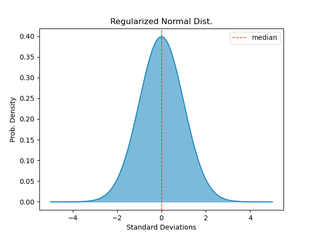
Our first distribution to test with is (as always) the normal distribution:
To get a handle on the practicality of this method, I simulated using it with up to five random data points. The results were somewhat surprising to me. In particular, I found that the widths of the min-to-max ranges increased (i.e. shifted rightward) much less with additional samples than I would have expected. Additionally, I was surprised to see that what shifts did appear seemed almost entirely to be associated with the elimination of smaller ranges that did not include the population median. On reflection, this makes sense since larger ranges should be more likely to capture the true population median, but before the simulation, I had not yet fully worked that out.

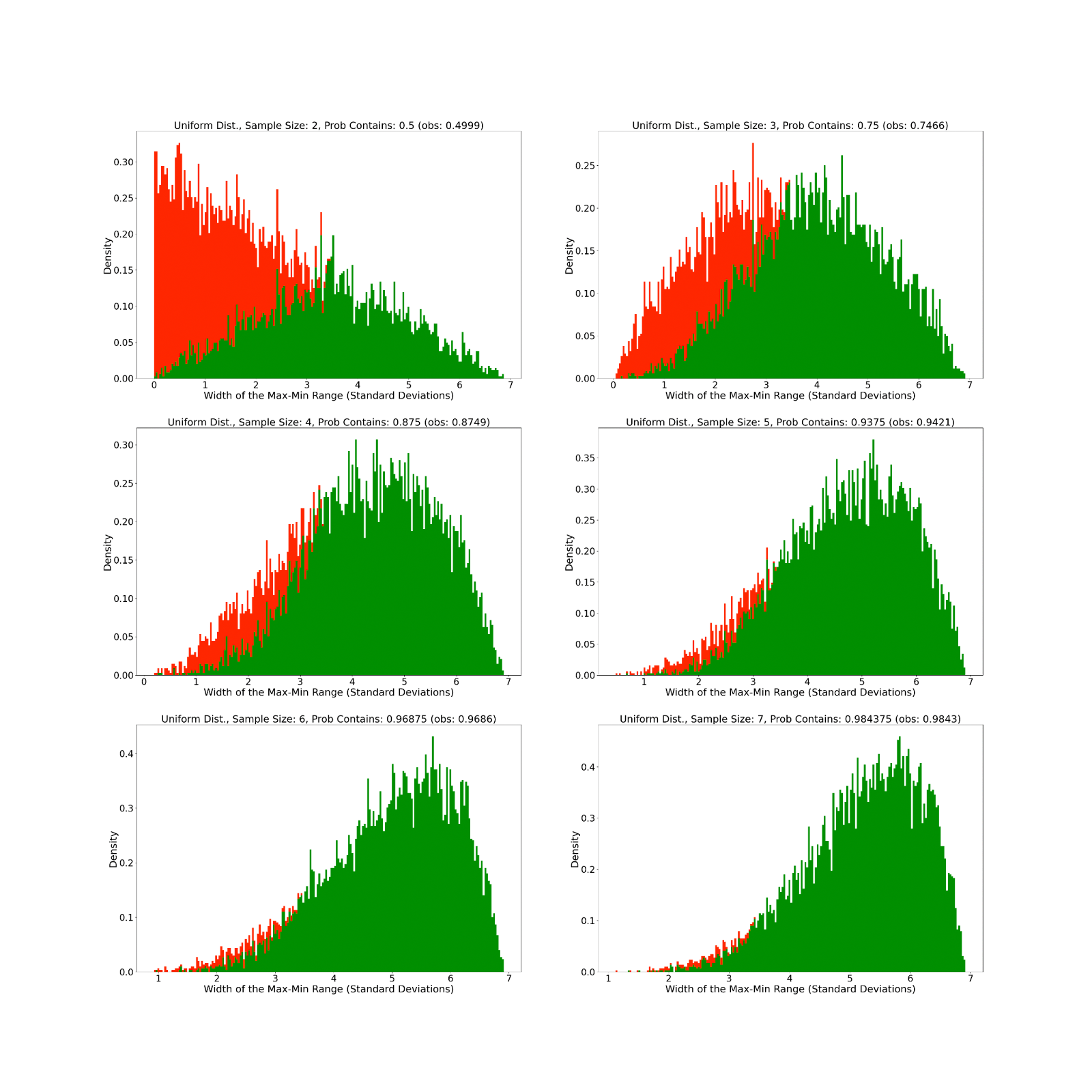
The Uniform Distribution
Our next distribution to simulate is the uniform distribution. Here, I think we see much more of a rightward shift to larger min-to-max ranges than with the normal distribution, though I am still not sure exactly why.

The Exponential Distribution
Our last distribution to simulate is the exponential distribution. This one surprised me since the bulk of min-to-max ranges actually stayed within a reasonable width, even as samples increased.


Final Thoughts
Those were all the simulations I did. I could definitely have done more, but I wasn’t sure what else I should try. If you have any ideas, then you should be able to (relatively) easily reuse my code on github for any distributions in the numpy.random library.
Anyway, I personally think this is a really cool bit of statistics that you can actually do in your head and explain to a normal person without a technical background. The practical usefulness of the method is somewhat debatable because of its sensitivity, but I still think that for at least a few distributions (normal, exponential), it is plausibly useful if you are very uncertain about the population you are sampling from and you only have a few (i.e. 5 or less) data points.
Technically, the probability can be greater or less than 50% for discrete variables, depending on the specific definition of median used and the discretization of the distribution, but I will ignore that here for simplicity.
Of course, this only applies for n > 1 since a number cannot be both below and above the median.
I don’t know if the combination would technically be considered more sensitive or not, but certainly in practical terms, it seems to combine the drawbacks of both.
I guess the next step might be finding the probability of n-1 out of n observations all being above (below) the median and then try to figure out how many observations you would need to have a 95% confidence in the median being between the second highest and second lowest observation.
I guess if you did this iteratively you could find an algorithm along the lines of: "With m independent observations the median is with 95% confidence between the k highest and k lowest observation."